
Nowadays most of the laser manufacturers provide the possibility to store the full waveforms in real time. After an Airborne LiDAR campaign it is therefore possible to apply more sophisticated algorithms to reach a deeper insight of the survey data.
The data collection is done, e.g., with the Riegl Laser VQ-880-G which stores the full waveform in a so called RXP-File(s). The necessary data content needed for further processing within a RXP-File are the recorded waveforms, direction vector together with the laser shot and receiver time. These files will be converted into a F5/HDF5 format which is the basic file format for further processing in HydroVISH.
The first step in the process chain is a peak detection ( Peak Detection) to transform the waveforms in some meaningful xyz-coordinates of the survey area. Due to the high measurement rates of the laser system the range ambiguity is then solved via MTA (Multiple Time Around) processing. Finally, a transformation from scanner coordinates to the appropriate desired coordinate system is deployed in HydroVISH to get the final point cloud ( Georeferencing).
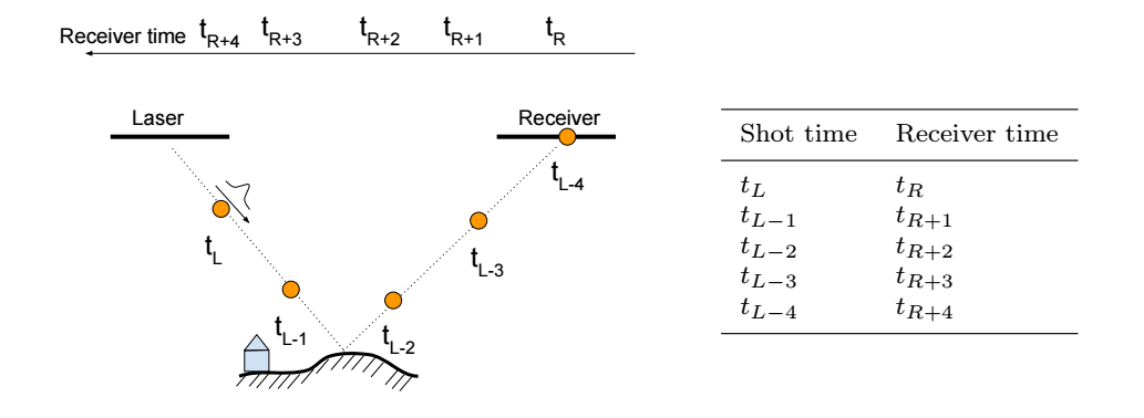
The resulting peaks derived from the full waveforms in ( Peak Detection) are used to calculate the range between start and end of the emitted pulse. Due to the high measuring rate of the Riegl-Laser (for VQ-880-G it is 550 kHz or 272 m as one way-length) a range ambiguity may occur. The problem is illustrated in Fig. 1 Multiple incoming laser shots traveling through the air until the hit the receiver. If the receiver is triggered at time tR to record a waveform it will automatically store the last laser shot (tL ). This leads to a wrongly calculated range length because of the time difference (tR- tL) . The true time couple for this example would be: tR - tL-4 and is also denoted as MTA 4. If the time coupletR - tL represent indeed the right range length of a different measurement this would be called: MTA 0 (only one shot traveling in Fig. 1})
|
|
| Fig.1 Left: Sketch of shot and receiver time. Right: Times stored in RXP-File. At receiver time tR the last shot time tL is stored together. The right time couple is supposed to be tR with tL-4, MTA Zone 4. |
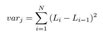
To overcome the range ambiguity the range measurement is calculated for all possible MTA - Zones. For every zone a circular buffer with size N is deployed to calculate the variance of consecutive range measurements. Therefore, for each MTA-Zone at current range measurement Lj the variance
|
is calculated within the circular buffer (i starts at i= j-N/2). Best results are archived with buffer length N = 50 which is particularly needed due to the high natural variation in vegetational area. The range measurement L at location j with the lowest variance of all MTA Zones is the correct one as shown in Fig.2, with resulting MTA-Zone 4. For the next range measurement Lj+1 the procedure is repeated. To improve the computational speed the equation for the variance is slightly modified: Instead of recalculating again the entire circular buffer for each range measurement only the newly create squared difference of (Li - Li-1)^{2} $ will be added to the buffer and the old variance will be subtracted.
In Fig. 2 the entire point cloud is recalculated for 6 different MTA-Zones, that is, the entire range measurement is calculated, with a fixed MTA-Zone, for example, MTA Zone 1 (time difference tR with Ltsub>L-3 in Fig. 1 or violet color in Fig. 2. If all MTA Zone are processed accordingly, MTA Zone 4 hast the lowest variance of range length. All other zone looks much more distorted and scattered than MTA Zone 4.

|
| Fig.2 6 different MTA-Zones: Orange MTA 0, violet MTA 1, black MTA 2, red MTA 3, green MTA 4 and blue MTA 5. MTA-Zone 4 (green-color) is the true zone with a slight transition zone at nadir (red color). |
As already indicated in Fig. 2 a MTA-Transition may occur. This happens when instead of 5 an additional 6th laser shot is traveling through the air for a short time and then again 5 laser shots (Fing. 1). This is sometimes an alternating process (e.g. from Zone 5 to 6 than back to 5) and a variance calculation as shown with the equation for the variance will result in many wrongly identify MTA-Zones for each range measurement. To solve this problem an additional buffer is defined with the functionality to calculate the variance with range measurements from previous (MTA-1) and post MTA-Zones (MTA+1). The Overlap of ± 1 handles now the transition zones: For example, in Fig. 2, at nadir some of the green points of MTA-Zone 4 (laser shot tL-4 in Fig. 1) move to Zone 5 (blue points) due to MTA transition and the resulting variances will be error prone. Instead, if each point form MTA-Zone 3 (red points) will be tested in MTA-Zone 4 (green points) there is at nadir a zone where these points match much better (low variance). Thus, with an overlap of ± 1 any possible transition zone can be solved.
Although, the buffer with overlap ability is theoretically sufficient to handle any transition zones a buffer with no overlapping is still needed. I some rare case - due to flaw range measurements - the buffer with overlap will become faulty and is therefore overwritten by the content of the non overlapping buffer. Additionally, for reliably MTA results, it is also necessary that the range measurement is indeed consecutive: For example, the Riegl-Laser VQ 780i delivers straight parallel scan lines from left to right in flight direction. This means a discontinuity when the scan line starts again at the left side. To improve the performance of the buffers it is therefore essential to flip every second scan line to get again continuous, consecutive lines.
MTA Zone: If negative the MTA zone will be calculated automatically; otherwise the MTA zone will be fixed according user input (e.g. 1 or 4, etc). MTA Zone starts with 0!
Data Type: With the imported RXP-File ( RXP import) two data sets are available: Automatically calculated points from the online processing (laser device) and its recorded waveforms . For both or for each individually a MTA processing can be deployed depending on the radio button "Data Type". For example, if "Skip FWF" is selected only Online Points will be processed. If "No Skip" is activated all waveforms are processed and online points will only be added if no recorded waveforms are available.
Export FWF: Adds corresponding waveform to every point).
Peak Detection: So far for methods are implemted: