Start Page
Point Cloud Extraction
Introduction:
Nowadays most of the laser manufacturers provide the possibility to store the full waveforms in real time.
After an Airborne LiDAR campaign it is therefore possible to apply more sophisticated algorithms to reach a deeper insight of the survey data.
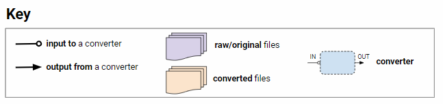
The data collection is done, e.g., with the Riegl Laser VQ-880-G which stores the full waveform in a so called RXP-File(s).
The necessary data content needed for further processing within a RXP-File are the recorded waveforms,
direction vector together with the laser shot and receiver time. These files will be converted into a F5/HDF5 format
which is the basic file format for further processing in HydroVISH.
The first step in the process chain is a peak detection to transform the waveforms in some meaningful xyz-coordinates of the survey area. Due to the high
measurement rates of the laser system the range ambiguity is then solved via MTA (Multiple Time Around) processing. Finally, a transformation from scanner
coordinates to the appropriate desired coordinate system is deployed in HydroVISH to get the final point cloud.
Peak Detection
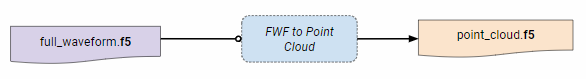
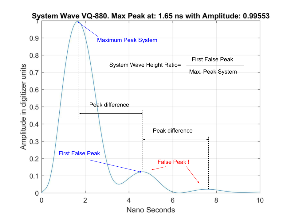
The recorded full waveform is typically a convolution of the system respond wave (Fig. 1) and the target cross section. This means that the waveform
is somehow smeared and the spatial resolution of the signal is decreased. Theoretically, to recover the original target signal a deconvolution of the system wave with the full waveform has to be done.
Many techniques are published to restore the original target cross section, for example B-splines, Wiener filter, Richardson-Lucy or exponential decomposition. In HydroVISH
we have been using the well known and reliable Gaussian Decomposition, among others, algorithm.
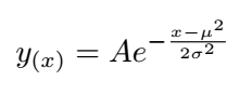
The basic idea behind the Gaussian Decomposition is to fit multiple gaussian shapes in the form of:
|
|
Fig.1 System Waveform (Riegl VQ 880-G).
|
into the waveform; whereas A is the amplitude, μ the mean value and σ the pulse width or standard deviation. The procedure in HydroVISH consist therefor of following steps:
- Estimation of peak positions via zero crossing of the derivated signal. The full waveform signal will be shifted to suppress peak detection in noisily region.
- With estimated peak positions a linear fitting (with three neighboring points of the signal) are carried out to estimate all parameters ($Amplitude$, $\mu$ and $\sigma$) of the gaussian shapes
- The estimated parameters ($Amplitude$, $\mu$ and $\sigma$) are further improved by using a non-linear best fitting algorithm (Levenberg-Marquardt).
- Subtracting superpositioned gaussien shapes from the full waveform. If the subtracted signal is still above noise level fitting process will be repeated
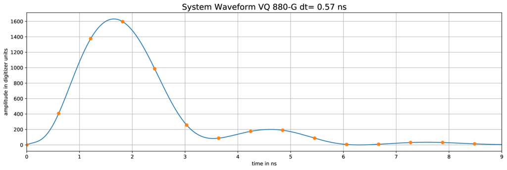
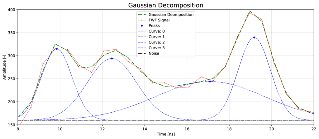
Fig. 2 shows an example of Gaussian Decomposition: The red line is the measured waveform with four detected peaks.
These peaks will be optimized with the Levenberg-Marquardt non-linear solver to calculate the four gaussian shapes (blue line).
If these shapes are superpositioned a similar curve as the full waveform is revealed and the fitting process is finished.
With the resulting parameter $Amplitude$ and σ further investigation for classification or roughness estimation are possible;
the parameter μ however is essential to determine the rang of the laser shot. With the temporal starting point of the waveform and the sampling interval
of the laser system (for VQ-880-G it is 0.57~ns) a range measurement can be determined for each peak of the full waveform. The last remaining
step is to remove some false detected peaks due to the after-pulse effect of the system wave (Fig. 1)
at time ≈ 4.5 and 7.5 ns. With the known peak heights and distances relatively to the main peak those range measurements can be easily deleted.
|
|
Fig.2 Gaussian Decomposition with the superposition of 4 gaussian shapes.
|
Comparison: Linear- and non linear Peak Fitting
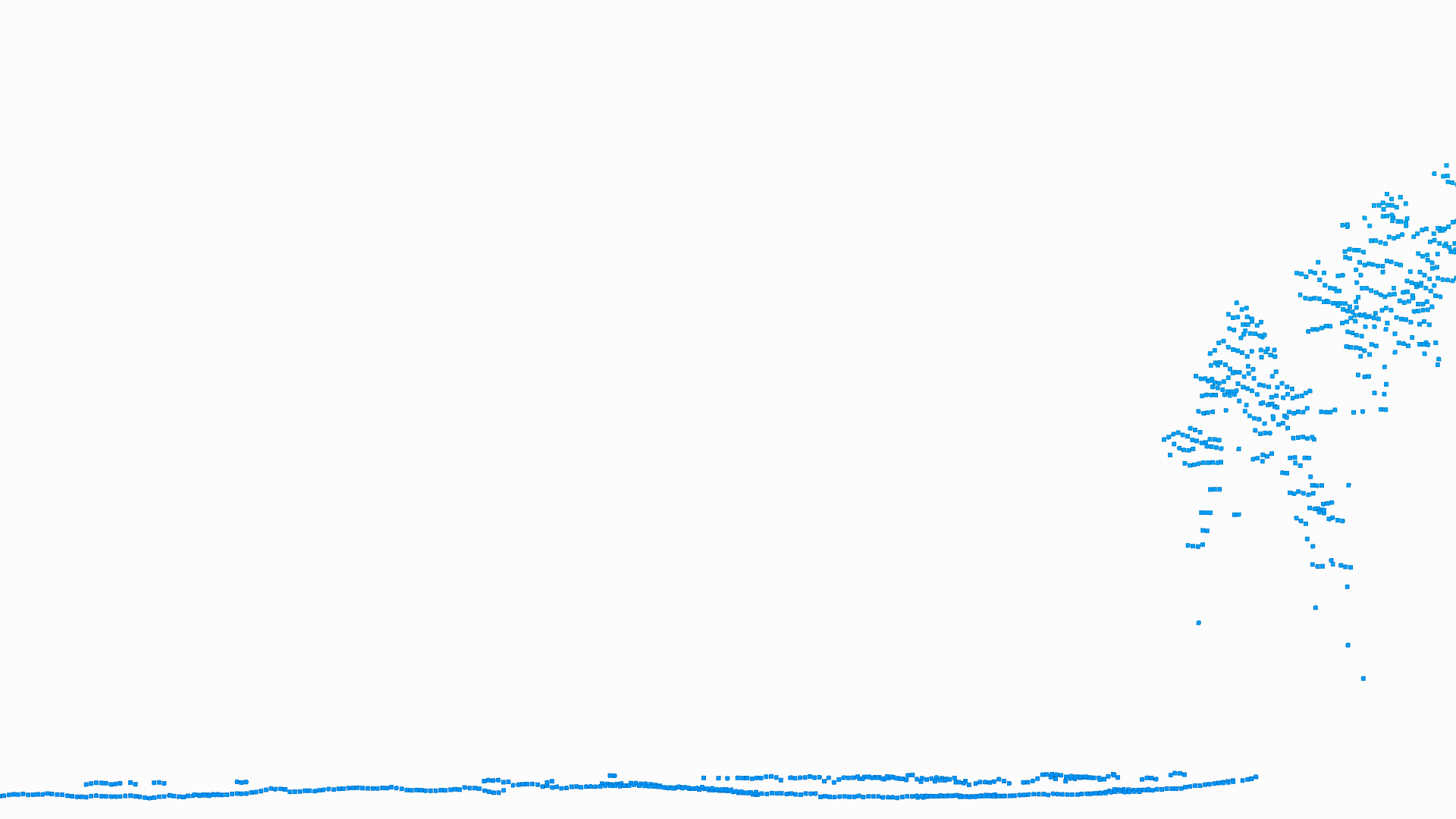
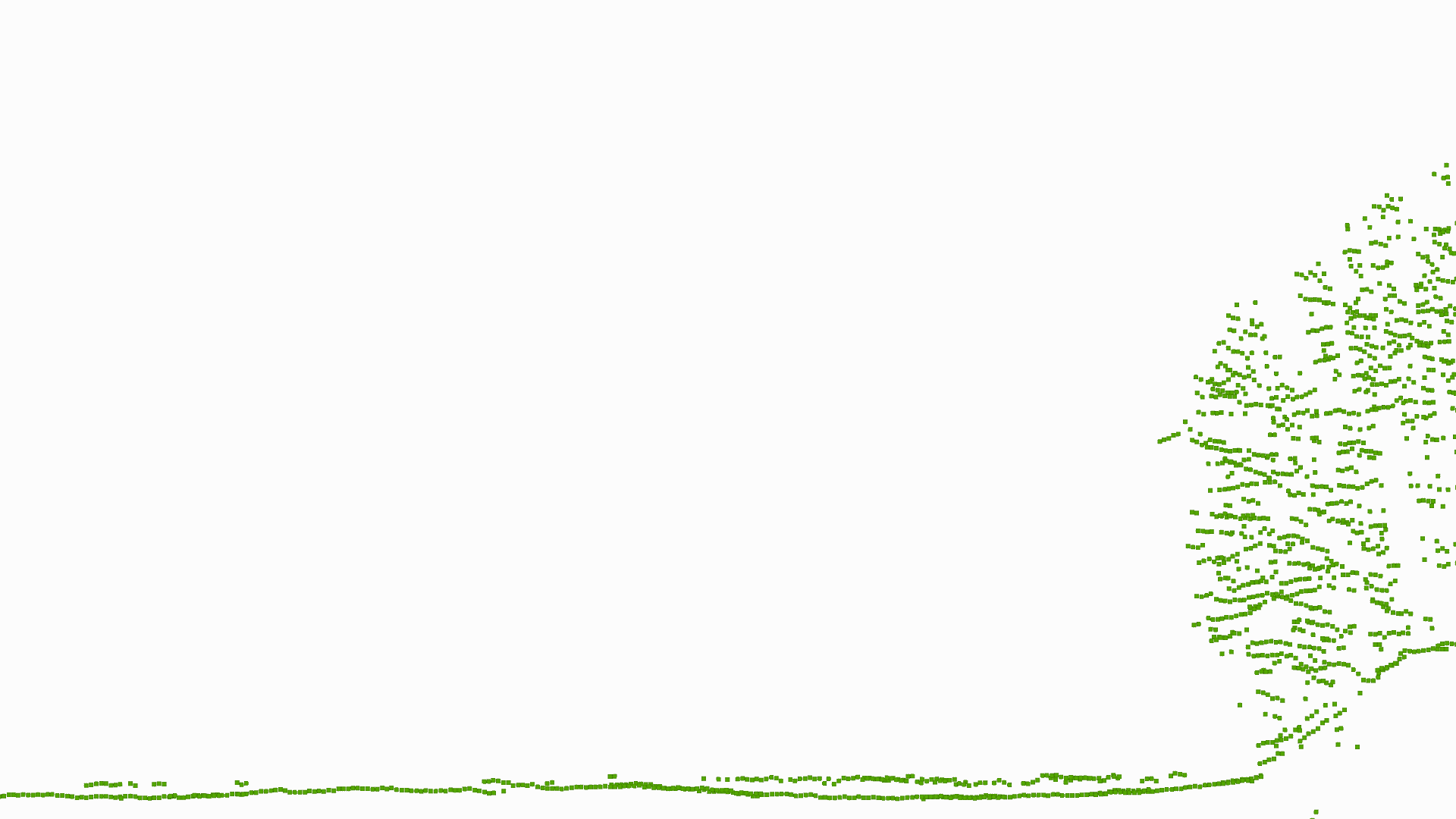
Fig. 4 and Fig. 5 visualize the difference between linear and non-linear fitting (see also item 2 and 3 in list above). Starting point is the online processed point cloud (Fig. 3) then follows (Fig. 4)
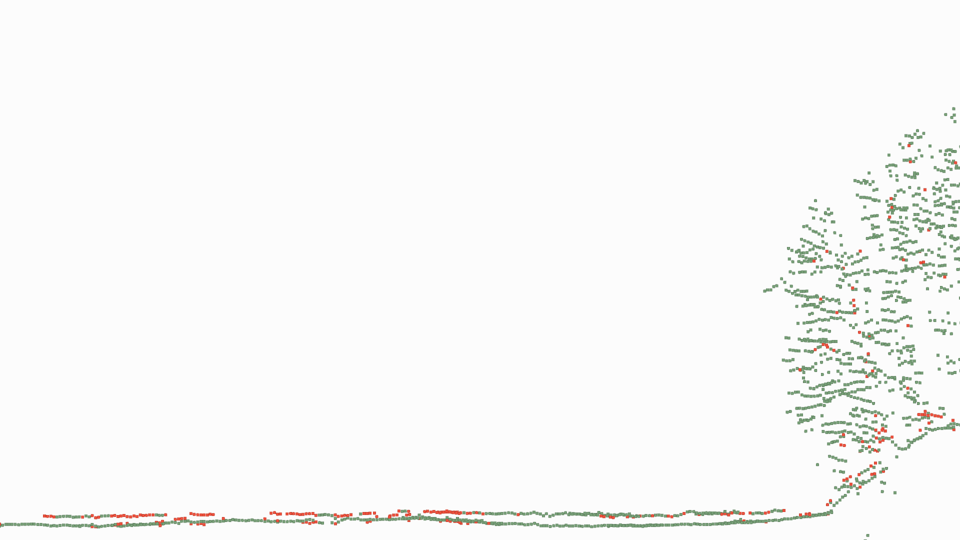
a linear fitting where the spatial accuracy is similar to the online processing (less than 10 cm). Finally, with the peaks of the linear fitting a non-linear calculation is done (Fig. 5). The result shows - beside spatial increasing accuracy -
additional "hidden" points (see red points in Fig. 5), naturally in areas where peaks are close together (e.g. water surface and river bed).
|
|
Fig.3 Gaussian Decomposition with superpositions of 4 gaussian shapes.
|
|
|
Fig.4 Gaussian Decomposition with superpositions of 4 gaussian shapes.
|
|
|
Fig.5 Gaussian Decomposition with superpositions of 4 gaussian shapes.
|
Options:
Noise level: Threshold to distinguish between noise and data. It is mostly close to the amplitude of 160 for VQ880. Noise level which is too
low results in many non existing points. If the noise level is too high river bed points can not be found.
Peak Detection: So far for methods are implemted:
- Linear Guass (LG): A fast and robust detection. Fits a Gaussian Shapes for three consecutive points.
- Gaussian Decomposition (GD): Gives some extra attributes like pulse-width. Peak detection resolution is better (two peaks close together yields still two peaks)
- Deconvolution (RL): See Richardson–Lucy deconvolution
- Hybrid: Blending between GD (for higher amplitudes) and RL (for lower amplitudes). Method with the best result but ~7 times slower than LG
System Wave Peak Difference: Depending on your system wave this is the distance (bin-unit) between the first main peak and the next smaller one (For VQ880 it is ~6, see Fig. 3).
System Wave Hight Ratio: Depending on your system wave this is the hight ratio between the first main peak and the next smaller one (For VQ880 it is ~0.5, see Fig. 3).
|
|
Fig.3 System wave with additional peaks after the maximum peak.
|
Back ¦
Start Page